The Complete Guide to 10 Python AI Libraries: Every Stage of a Quant Trading Workflow
A one-stop guide to the positioning of 10 core Python AI libraries in quantitative trading: NumPy for numerical computing, pandas for financial time series, scikit-learn for traditional ML, XGBoost/LightGBM as the workhorses for tabular data, PyTorch for research-oriented deep learning, TensorFlow/Keras for production deployment, and Jupyter as the research environment—plus practical use cases for statsmodels, spaCy, Transformers, backtrader, vectorbt, ccxt, MetaTrader5, and TA-Lib. Includes typical installation combinations and a decision tree.
Why Write This Article?
Stepping into quantitative trading, Python is the default language—but "Python" as an answer is too vague. A complete ML / quant workflow uses at least 5 distinctly different libraries:
- Numerical computing → NumPy
- Data cleaning → pandas
- Traditional ML → scikit-learn
- Time series / statistical models → statsmodels
- Gradient Boosting (the king after feature engineering) → XGBoost / LightGBM / CatBoost
- Deep learning → PyTorch or TensorFlow + Keras
- NLP / sentiment analysis → HuggingFace Transformers / spaCy
- Backtesting → backtrader / vectorbt / custom
- Live trading → ccxt / broker API / MetaTrader5
- Research environment → Jupyter / VSCode
The goal of this article is to master the positioning, use cases, and quant-trading practical applications of these 10 libraries in one read. After reading, you should know how to choose: "What should I import at this moment?"
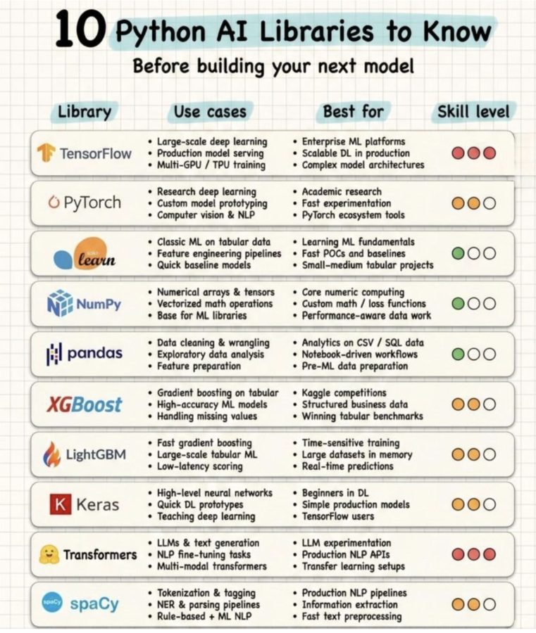
The accompanying cheat sheet (cover image) for this article will appear once more at the end.
1. Overall Workflow: Where Each Library Fits
A typical quant strategy pipeline:
Raw data (CSV / Parquet / DB)
    ↓
[ pandas ]      Cleaning, resampling, feature engineering
    ↓
[ NumPy ]       Vectorized computation, rolling statistics
    ↓
[ scikit-learn ]  Baseline ML, feature selection, pipeline
    ↓ (optional)
[ XGBoost / LightGBM / CatBoost ]  Tabular ML workhorse
    ↓ (optional)
[ PyTorch / TF-Keras ]  Time series models, CNN, Transformer
    ↓
[ Custom backtest / backtrader / vectorbt ]  Backtest
    ↓
[ Broker SDK / MT5 ]   Live trading
    ↓
[ Jupyter / VSCode ]  Exploration + documentation
Core principle: 80% of the time is spent inside pandas + NumPy. Other libraries are the "final decision-makers," but the first 80% of code is ETL.
1.1 Two Dimensions for Choosing a Library
| Dimension | Selection Criteria |
|---|---|
| Data type | Numeric/vector → NumPy; tabular → pandas; time series → pandas + statsmodels; text → spaCy/Transformers; images → PyTorch/TF |
| Task type | Linear models → sklearn; tree models → XGBoost/LightGBM; DL models → PyTorch/TF; NLP → Transformers; backtesting → backtrader/vectorbt |
These two dimensions determine 90% of import choices.
2. NumPy — The Root of Numerical Computation
Purpose: N-dimensional arrays, vectorized math, linear algebra, random numbers, boolean masking.
How it's used in quant trading:
- ATR, EMA, RSI written in NumPy run 10-100x faster than pandas
- Any "rolling calculation" you find too slow in pandas can be implemented at the NumPy level using
np.lib.stride_tricks.sliding_window_view - Foundation for custom indicators and feature functions
Typical installation:
pip install numpyQuant example: Computing ATR with NumPy:
import numpy as np

def atr_numpy(high, low, close, period=14):
    prev_close = np.concatenate([[close[0]], close[:-1]])
    tr = np.maximum.reduce([
        high - low,
        np.abs(high - prev_close),
        np.abs(low - prev_close)
    ])
    return np.convolve(tr, np.ones(period) / period, mode='valid')
Quant reminder: pandas is built on NumPy internally, so most of the time you don't need to explicitly import numpy. But when writing low-level signal engines, using NumPy directly avoids performance issues and bugs caused by pandas index.
3. pandas — The Standard Container for Financial Time Series
Purpose: Table cleaning, resampling (5min → 1H), rolling, groupby, merge.
How it's used in quant trading:
- Read CSV / Parquet
- Compute OHLCV-derived columns
- Resample to different timeframes
- Join multiple symbols, build cross-sectional features
Typical installation:
pip install pandas pyarrowQuant example:
import pandas as pd
df = pd.read_parquet('XAUUSD_M5.parquet')
df['returns'] = df['close'].pct_change()
df['atr'] = df['high'] - df['low']  # simplified version
df_hour = df.resample('1H').agg({
    'open': 'first', 'high': 'max', 'low': 'min', 'close': 'last', 'volume': 'sum'
})
Quant reminder: Thepyarrowbackend in pandas 2.x processes large data 5-10x faster. For 500MB+ time series data, rememberdtype_backend='pyarrow'.
4. scikit-learn — The Entry Ticket to Traditional ML

Purpose: train/test split, StandardScaler, linear/ridge/lasso/elasticnet, RandomForest, SVM, PCA, KMeans, cross_val_score, GridSearchCV, Pipeline.
How it's used in quant trading:
- Feature standardization (
StandardScaler) - Cross-validation (
TimeSeriesSplit— don't use regular KFold) - Simple classification / regression baselines
- Feature selection (
SelectKBest,Lasso) - Pipeline chaining for multi-step processing
Typical installation:
pip install scikit-learnQuant example — Time-series cross-validation:
from sklearn.model_selection import TimeSeriesSplit
from sklearn.ensemble import RandomForestClassifier
from sklearn.pipeline import Pipeline
from sklearn.preprocessing import StandardScaler

tscv = TimeSeriesSplit(n_splits=5)
pipe = Pipeline([
    ('scaler', StandardScaler()),
    ('clf', RandomForestClassifier(n_estimators=200, max_depth=5))
])
for fold, (train_idx, test_idx) in enumerate(tscv.split(X)):
    pipe.fit(X.iloc[train_idx], y.iloc[train_idx])
    score = pipe.score(X.iloc[test_idx], y.iloc[test_idx])
    print(f"Fold {fold}: {score:.3f}")
Quant reminder: Never usetrain_test_split(random_state=...)— it leaks future data. Always useTimeSeriesSplit.
5. TensorFlow + Keras — The First Choice for Production Deployment

Purpose: Deep learning models, production serving (TFX, TF Serving), multi-GPU / TPU training.
How it's used in quant trading:
- LSTM / GRU time series models
- Transformer encoder for sequence-to-sequence prediction
- Cross-asset feature learning
- Large-scale training (if not on a laptop)
Typical installation:
pip install tensorflowQuant example — Building an LSTM with Keras:
import tensorflow as tf
from tensorflow.keras import layers, Model

inputs = layers.Input(shape=(60, 5))  # 60 bars, 5 features
x = layers.LSTM(64, return_sequences=True)(inputs)
x = layers.LSTM(32)(x)
x = layers.Dense(16, activation='relu')(x)
out = layers.Dense(1, activation='sigmoid')(x)  # up / down

model = Model(inputs, out)
model.compile(optimizer='adam', loss='binary_crossentropy', metrics=['accuracy'])
Quant reminder: TF 2.x is actually slower than PyTorch for small research projects (eager mode overhead is large). If you're only doing research, not production serving, just pick PyTorch.
6. PyTorch — Research and Rapid Experimentation

Purpose: Deep learning research, custom model architectures, reinforcement learning, dynamic graphs.
How it's used in quant trading:
- Custom loss functions (e.g. Sharpe ratio loss)
- Reinforcement learning strategies
- GAN / VAE for synthetic financial data
- Cross-frequency attention models
Typical installation:
pip install torch torchvision torchaudio  # CPU
# GPU: go to the official site and pick the matching CUDA version
Quant example — Sharpe-ratio loss function:
import torch
import torch.nn as nn

class SharpeLoss(nn.Module):
    # Negative Sharpe ratio as loss. Minimize = maximize Sharpe.
    def forward(self, returns):
        # returns: shape (batch, time)
        mean = returns.mean(dim=-1)
        std = returns.std(dim=-1) + 1e-8
        sharpe = mean / std
        return -sharpe.mean()
Quant reminder: PyTorch's dynamic graph makes debugging super easy — any print(model(x)) directly gives you the shape and values of intermediate tensors.7. Jupyter Notebook — The Playground for Research
Purpose: Interactive Python, Markdown notes, inline charts, sharing research results.
How it's used in quant trading:
- Exploratory data analysis (EDA)
- Rapid prototyping
- Writing research journals for future reference
Typical installation:
pip install jupyterlab ipywidgetsQuant example — Inline backtest plot:
import pandas as pd
import matplotlib.pyplot as plt

%matplotlib inline
df = pd.read_parquet('XAUUSD_H1.parquet')
df['close'].plot(figsize=(14, 5), title='XAUUSD H1')
plt.show()
Quant reminder: Jupyter is great, but production code should not live inside notebooks. Notebook hidden state (residual variables, cell-order dependencies) is a production nightmare.
8. XGBoost — The Killer Weapon for Tabular Data
Purpose: Gradient boosting, tabular data, Kaggle competition-level performance.
How it's used in quant trading:
- Workhorse model for structured features (OHLCV + indicators + macro)
- Cross-sectional alpha prediction across symbols
- Mid-frequency signals (5min-1D)
Typical installation:
pip install xgboostQuant example:
import xgboost as xgb

dtrain = xgb.DMatrix(X_train, label=y_train)
dtest = xgb.DMatrix(X_test, label=y_test)
params = {
    'objective': 'binary:logistic',
    'max_depth': 5,
    'learning_rate': 0.05,
    'subsample': 0.8,
    'colsample_bytree': 0.8,
    'eval_metric': 'auc',
    'tree_method': 'hist',  # fast
}
model = xgb.train(params, dtrain, num_boost_round=200,
                  evals=[(dtest, 'test')], early_stopping_rounds=20, verbose_eval=10)
Quant reminder: XGBoost handles NaN automatically, runs fast, and is highly interpretable (plot_importance). The tabular baseline for financial time series must always start here.9. LightGBM — Big Data + Low Latency

Purpose: Similar to XGBoost, but trains faster, uses less memory, and is more friendly to large datasets.
How it's used in quant trading:
- Millions of rows of K-line + hundreds of features
- Needs rapid retrain (e.g. intraday rolling training)
- Large-scale cross-sectional training
Typical installation:
pip install lightgbmQuant example:
import lightgbm as lgb

train_data = lgb.Dataset(X_train, label=y_train)
test_data = lgb.Dataset(X_test, label=y_test, reference=train_data)

params = {
    'objective': 'binary',
    'metric': 'auc',
    'num_leaves': 31,
    'learning_rate': 0.05,
    'feature_fraction': 0.8,
    'bagging_fraction': 0.8,
    'bagging_freq': 5,
}
model = lgb.train(params, train_data, valid_sets=[test_data],
                  num_boost_round=500, callbacks=[lgb.early_stopping(20)])
Quant reminder: LightGBM vs XGBoost, which to pick? No standard answer. Generally LightGBM is faster on big data, XGBoost has a slightly higher Kaggle win rate. Try both.
10. Other Essentials (Quick Look)
These aren't top-10, but are must-haves in practice:
| Library | Purpose | Quant usage |
|---|---|---|
| statsmodels | ARIMA / GARCH / VAR | Classic time series models, cointegration test |
| HuggingFace Transformers | Pretrained LLM / NLP | Financial news sentiment, news classification |
| spaCy | Fast NLP pipeline | Named entity recognition (companies, people), text preprocessing |
| backtrader | Backtesting framework | Multi-strategy, multi-timeframe event-driven backtests |
| vectorbt | High-speed backtesting (vectorized) | Large-scale parameter sweep, portfolio backtest |
| ccxt | Unified crypto API | Unified interface for 100+ exchanges |
| MetaTrader5 | MT5 Python SDK | Forex / CFD live order placement |
| TA-Lib | 100+ technical indicators in C | Fast computation of RSI, MACD, Bollinger, etc. |
Philosophy for choosing libraries: Use the one you're most familiar with to solve 90% of the problems—don't chase the new one. The production risk of a new library always outweighs its performance advantage.
11. Typical Installation Combination
A standard requirements.txt for a quant trader / researcher:
# Core
numpy>=1.24
pandas>=2.0
scipy>=1.10

# Traditional ML
scikit-learn>=1.3
statsmodels>=0.14

# Gradient Boosting
xgboost>=2.0
lightgbm>=4.0
catboost>=1.2  # handles categorical features

# Deep Learning
torch>=2.0  # or tensorflow>=2.13

# NLP
transformers>=4.30
spacy>=3.6

# Backtesting / Trading
backtrader>=1.9
vectorbt>=0.25
ccxt>=4.0
MetaTrader5>=5.0  # Windows only

# Research tools
jupyterlab>=4.0
matplotlib>=3.7
seaborn>=0.12
plotly>=5.15
Installation tip: Use pip install -r requirements.txt, don't use Anaconda (too many dependency conflicts). For CUDA, use the official conda install pytorch cudatoolkit=11.8 -c pytorch.
12. How to Decide What to Import?
Decision tree:
- Loading + cleaning → pandas
- Vectorized computation → NumPy
- Baseline ML → scikit-learn
- Strong tabular model → XGBoost / LightGBM
- Time series / DL → PyTorch (or TF + Keras)
- NLP → spaCy (fast) / Transformers (strong)
- Backtesting → backtrader (event-driven) / vectorbt (fast)
- Live trading → Broker SDK
- Exploration → Jupyter
- Production → VSCode + git + pytest
Common mistake: Using PyTorch to run a 10K-row CSV. DL on small datasets (< 100K rows) almost always loses to XGBoost. Start with sklearn baseline, then XGBoost, and only consider DL last.
13. Conclusion
These 10 libraries don't mean "you must master all of them," but rather "at least know what they do, why they exist, and who uses them." The reality of quant trading is:
- 80% of the time: pandas + NumPy
- 15% of the time: sklearn + XGBoost / LightGBM
- 4% of the time: PyTorch / TF
- 1% of the time: NLP, special libraries
Remember: libraries are tools, not identities. Knowing how to use more libraries doesn't make you stronger; knowing how to pick the most fitting one is the real skill.
Things you can do next:
- Run
pip list --outdatedto upgrade your current environment - Write a
requirements.txtto lock versions, avoid the "but it works on my machine" tragedy - Pass backtest results and ML signals using the same dict structure, avoid type confusion
- Consider using
poetryoruvto replacepipfor more stable dependency management
Cover image cheat sheet for this article (positioning of the 10 major libraries):
⚠️ Disclaimer: This article is for educational purposes only and does not constitute investment advice. Investing involves risk.